Heart Disease Risk Prediction
Classic ML modeling and resampling with R: A deep dive
Introduction
Within the limits of this Kaggle dataset of heart disease indicators, we’ll employ and compare two supervised learning models (logistic regression and random forest) for binary prediction. As we will discuss later, imbalance in the data will necessitate resampling, and two techniques (undersampling and ROSE) will be tested against each other as well.
We want to answer the question:
What are the biggest contributors to heart disease?
Load Libraries and Data
The biggest issue with this dataset is the predictor variable class imbalance:
> table(heart$HeartDiseaseorAttack)
      0      1
229787  23893
229,787 zeros (Does not have heart disease or had an attack) and 23,893 ones (Does have).
Exploratory Data Analysis
Grid Plot of Binary Data
The R Code
The Plot
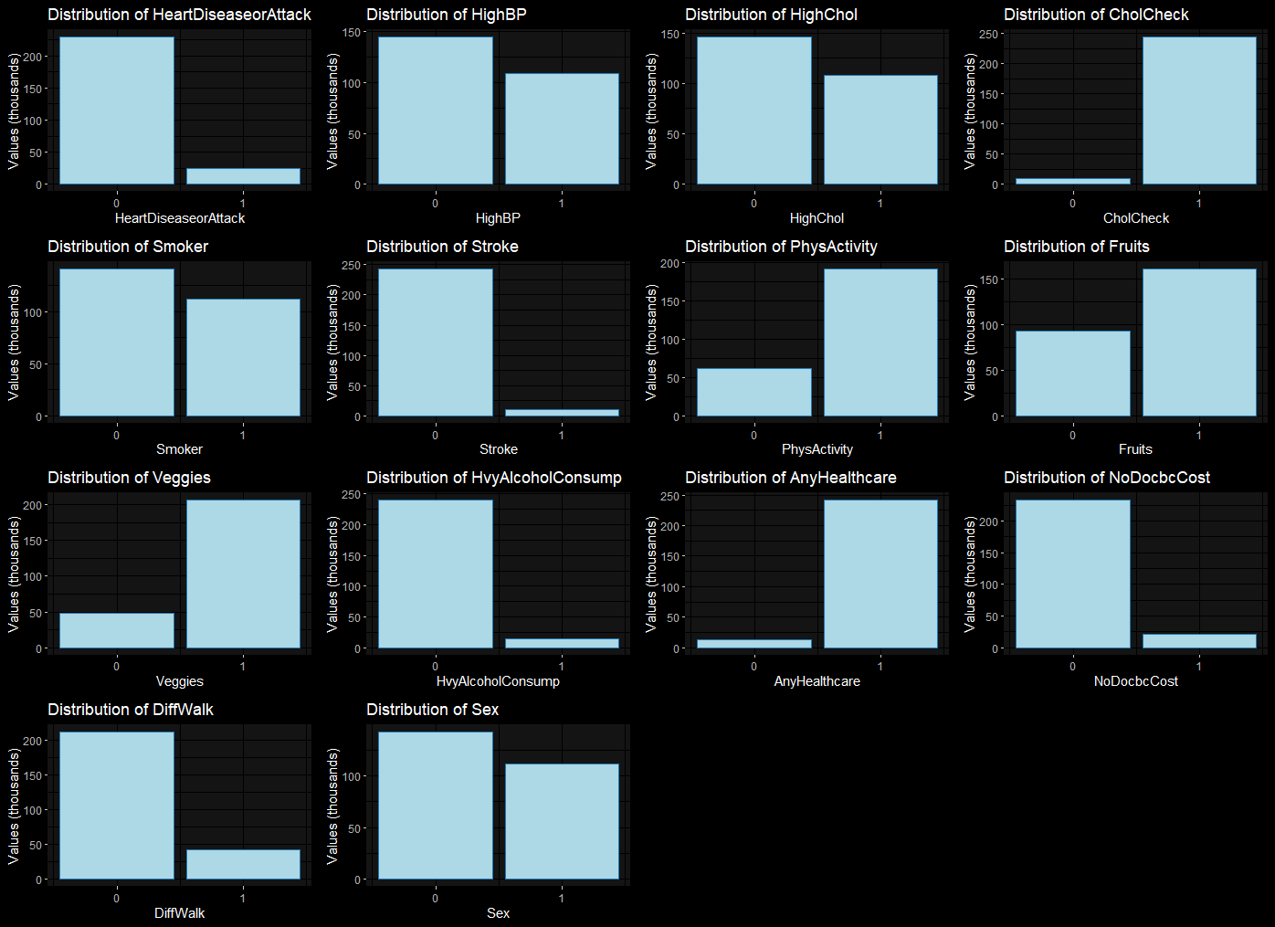
There are a number of features where either zero or one are predominant, indicating they may be of little predictive value. We need to keep an eye on CholCheck, Stroke, Veggies, and the other imbalanced features.
Non-Binary (Continuous) Data Box Plot
The R Code
ggplot(heart_non_binary_long,
       aes(x=Variable, y=Value)) +
  geom_boxplot(fill = 'lightblue', color = '#1F78B4') +
  labs(title = 'Box Plot',
subtitle = 'Non Binary Value Columns')The Plot
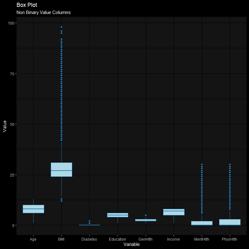
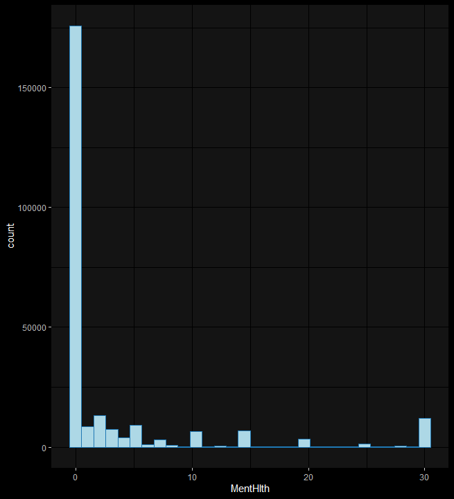
There are issues that need attention here: Big outliers in BMI and abnormal distributions in MentHlth and PhysHlth, something mysterious about the values in the Diabetes column, which should be either 0 or 1:
> table(heart$Diabetes)
     0      1      2
213703   4631  35346
After some research, we discover the exact encoding from the original dataset:
- No diabetes or only during pregnancy
- Pre- or borderline diabetes
- Yes diabetes
We will convert this column into a factor (a grouping for categorical variables) later. On to the remaining non-binary data.
Inspection of Continuous Variables
Plan for Preprocessing
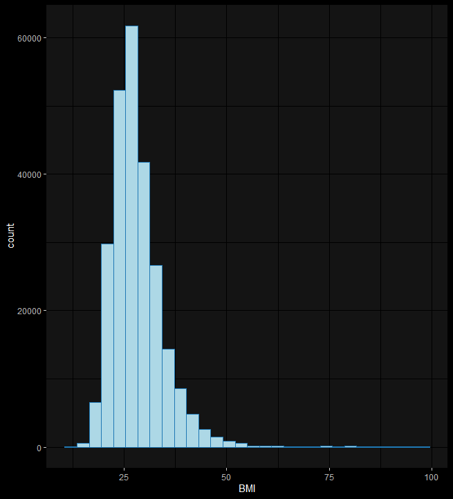
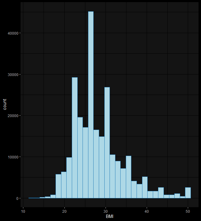
BMINeed to trim away values that are outside of the US distribution of values (> 50).
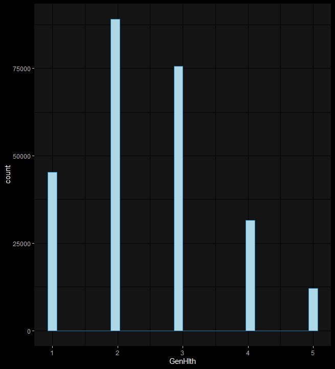
GenHlthThis needs to be a factor, not a continuous value.
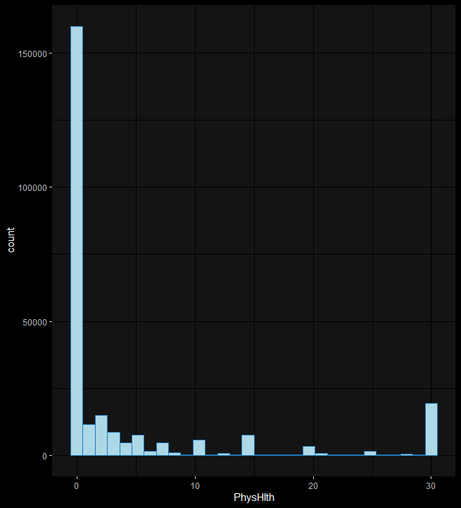
PhysHlth"Number of bad health days a month". Given this distribution, we'll split down the middle and convert to a binary value.
MentHlth"Number of bad mental health days a month". Treat the same as PhysHlth.
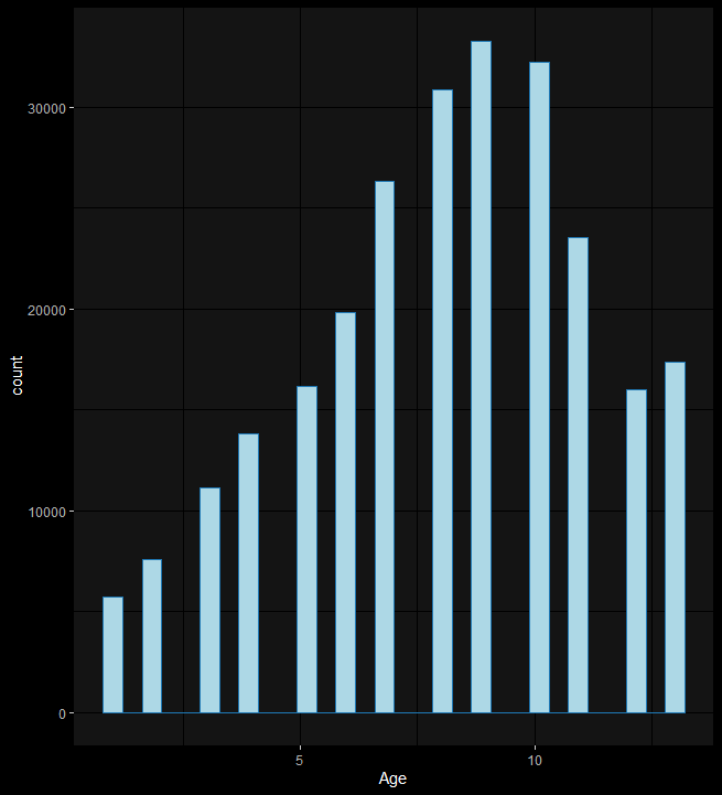
AgeConvert to factor, thusly: 1 = 18-24, 2 = 25-29, 3 = 30-34; by 5's.
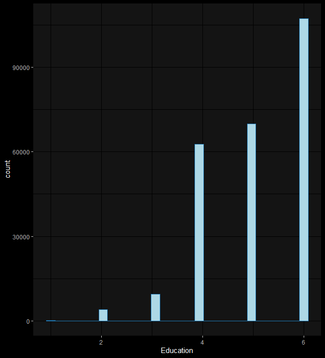
EducationTo factor: 1-6.
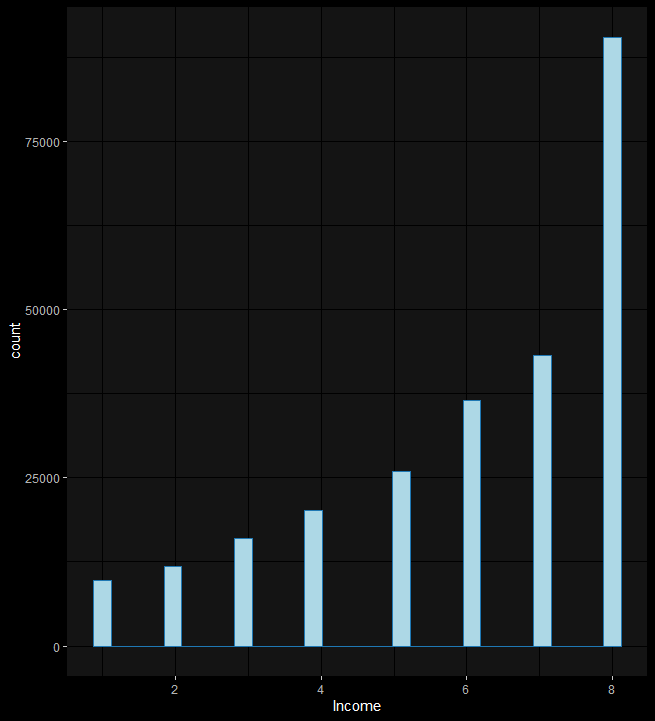
IncomeTo Factor: 1 = Less than $10,000, 2 = Less than $15,000, 3 = Less than $20,000, 4 = Less than $25,000, 5 = Less than $35,000, 6 = Less than $50,000, 7 = Less than $75,000, 8 = $75,000 or more.
BMI(After Trim)
Execute Preprocessing Plans
## CAP BMI:
heart$BMI <- ifelse(heart$BMI > BMI_limit, BMI_limit, heart$BMI)

## TURN GenHlth AROUND (1 POOR -> 5 EXC.):
heart$GenHlth <- (5 + 1) - heart$GenHlth

## TO BINARY -> SPLIT AT MID-MONTH
# PhysHlth and MentHlth
heart$PhysHlth <- ifelse(heart$PhysHlth >= 14, 1, 0)
heart$MentHlth <- ifelse(heart$MentHlth >= 14, 1, 0)

## CONVERT TO FACTOR:
# Diabetes
# GenHlth
# Age
# Education
# Income
cols_2_factor <- c('Diabetes', 'GenHlth', 'Age',
                   'Education', 'Income')
heart[cols_2_factor] <- lapply(heart[cols_2_factor], as.factor)Final Feature Engineering
First, we fit a logistic regression model with the full dataset and remove any clearly unnecessary features based on the results.
Fit Initial Logistic Regression Model
glm_fulldata <- glm(HeartDiseaseorAttack ~ ., data = heart,
                    family = 'binomial')
summary(glm_fulldata)Select Columns to Drop
BMI- One thing that jumps out is
BMI. Why, against expectations, is it not significant? After investigation, it turns out that in the presence of features that are connected toBMI(HighBP,HighChol,Diabetes),BMIitself is not predictive - drop it. R code:cols_to_drop <- c('BMI) GenHlthvs.PhysHlth- R code:
cor(as.numeric(heart$GenHlth), heart$PhysHlth) = -0.48. This is a big enough correlation and the latter is not significant, so let’s drop it.PhysActivity,Fruits, andVeggiesaren’t doing anything that isn’t covered byGenHlth, so let’s drop them too for the sake of explainability. R code:cols_to_drop <- append(cols_to_drop, c('PhysHlth', 'PhysActivity', 'Fruits', 'Veggies')) HvyAlcoholConsumpHvyAlcoholConsumpis significant and as a negative coefficient, indicates a reduction in risk. Why would drinking too much decrease the likelihood of heart disease? It turns out there is a known “Sick Quitter” effect, where people who get sick stop drinking. This is a bogus feature. R code:cols_to_drop <- append(cols_to_drop, 'HvyAlcoholConsump')AnyHealthcareandEducation- With very low statistical significance and near zero coefficent, both
AnyHealthcareandEducationare useless in the model. R code:cols_to_drop <- append(cols_to_drop, c('AnyHealthcare', 'Education'))
Drop selected columns and check the fit again
Every feature that remains is significant - we’re finally ready for modeling.
Modeling
Since the class imbalance is so severe (roughly 9 No’s to 1 Yes), there are some concerns that need to be addressed:
- Training on the whole dataset will teach the model that always guessing “NO heart disease” will be correct 90% of the time.
- Either “over” or “under” sampling (or both) needs to be done for the training data. For comparison’s sake, we’ll make two training sets: a. Undersampled - trim away the majority class until balanced, and b. “ROSE” (Random Over-Sampling Examples) which generates artificial data to balance the classes.
- BUT, testing on the balanced sets will make the models look like they perform better than they are, especially in terms of precision (true positives/all positive predictions).
Therefore, the plan is this - two models, two resampling techniques:
- Split the imbalanced data 70/30, keeping the imbalance.
- Create an undersampled training set (
train_under) and an oversampled one (train_rose). - Fit a Logistic Regression model and a Random Forest on both
train_underandtrain_rose. - Evaluate on the imbalanced 30% test_set from 1.
Split
set.seed(99)
train_index <- createDataPartition(heart$HeartDiseaseorAttack, p=0.7, list=F)
train_data <- heart[train_index, ]
test_data <- heart[-train_index, ]Compare Proportions
> prop.table(table(train_data$HeartDiseaseorAttack))

         0          1
0.90642317 0.09357683

> prop.table(table(test_data$HeartDiseaseorAttack))

         0          1
0.90439399 0.09560601
The test/train splits are of nearly equal proportion and are therefore acceptable.
Create Training Sets and Run Predictions
train_under <- ovun.sample(HeartDiseaseorAttack ~ ., data = train_data,
                           method = 'under')$data
train_under$HeartDiseaseorAttack <- as.factor(train_under$HeartDiseaseorAttack)

train_rose <- ROSE(HeartDiseaseorAttack ~ ., data = train_data,
                   seed = 99)$data
train_rose$HeartDiseaseorAttack <- as.factor(train_rose$HeartDiseaseorAttack)

# Fit and predict
glm_rose <- glm(HeartDiseaseorAttack ~ ., data = train_rose,
                     family = 'binomial')
glm_under <- glm(HeartDiseaseorAttack ~ ., data = train_under,
                     family = 'binomial')
rnd_forest_rose <- randomForest(HeartDiseaseorAttack ~ .,
                                 data = train_rose, ntree=500) # ⚠ little long! ⚠
rnd_forest_under <- randomForest(HeartDiseaseorAttack ~ .,
                                 data = train_under, ntree=500)

pred_glm_rose <- predict(glm_rose, test_data, type = 'response')
pred_glm_under <- predict(glm_under, test_data, type = 'response')
pred_rf_rose_yes <- predict(rnd_forest_rose, test_data, type = 'prob')[ ,2]
pred_rf_under_yes <- predict(rnd_forest_under, test_data, type = 'prob')[ ,2]Results
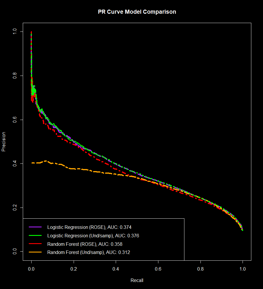
For this dataset the Area Under the Precision Recall Curve (AUC-PR) is the best way to rate/compare classification model performance as the data is highly imbalanced. It is particularly useful in our case, where the positive class is rare and when the cost of false positives and false negatives is high.
AUC-PR is Precision (the proportion of true positives among all positive predictions) against Recall (correctly identified true positives) at various threshold settings (the decision boundary of no/yes)
AUC-PR Implementation and Plot
# AUC-PR
test_data_labels <- ifelse(test_data$HeartDiseaseorAttack == 1, 1, 0)
pr_glm_rose <- pr.curve(scores.class0 = pred_glm_rose, weights.class0 = test_data_labels, curve = T)
pr_glm_under <- pr.curve(scores.class0 = pred_glm_under, weights.class0 = test_data_labels, curve = T)
pr_rf_rose <- pr.curve(scores.class0 = pred_rf_rose_yes, weights.class0 = test_data_labels, curve = T)
pr_rf_under <- pr.curve(scores.class0 = pred_rf_under_yes, weights.class0 = test_data_labels, curve = T)

# Build Comparative Plot
par(bg='black', fg='white', col.main='white', col.lab='white', col.axis='white')
plot(pr_glm_rose, main='PR Curve Model Comparison', col='purple', lwd=4, lty=5, auc.main=F, legend=F)
lines(pr_rf_rose$curve[ ,1], pr_rf_rose$curve[ ,2], col='red', lwd=4, lty=4)
lines(pr_rf_under$curve[ ,1], pr_rf_under$curve[ ,2], col='orange', lwd=4, lty=6)
lines(pr_glm_under$curve[ ,1], pr_glm_under$curve[ ,2], col='green', lwd=4, lty=3)
legend('bottomleft',
       legend=c(paste('Logistic Regression (ROSE), AUC:', round(pr_glm_rose$auc.integral, 3)),
                paste('Logistic Regression (Und/samp), AUC:', round(pr_glm_under$auc.integral, 3)),
                paste('Random Forest (ROSE), AUC:', round(pr_rf_rose$auc.integral, 3)),
                paste('Random Forest (Und/samp), AUC:', round(pr_rf_under$auc.integral, 3))),
col=c('purple', 'green', 'red', 'orange'), lwd=3)AUC-PR Comparison Plot
AUC-PR Comparison Table
Ranked Model Performance
| Rank | Model | Sample Method | AUC.PR | Notes |
|---|---|---|---|---|
| 1 | Logistic Regression | Undersampled | 0.376 | Simplest and best |
| 2 | Logistic Regression | ROSE | 0.374 | Same performance as 1, more memory req’d |
| 3 | Random Forest | ROSE | 0.358 | Slighly worse performance, computationally heavier |
| 4 | Random Forest | Undersampled | 0.312 | Poor, starved for data |
Calculated Odds by Predictor
odds_ratios <- as.data.frame(exp(coef(glm_under)))
or_desc <- odds_ratios %>%
  select('Odds.Ratio' = 'exp(coef(glm_under))') %>%
arrange(desc(Odds.Ratio))Odds Ratios (Greater than 1 = increased odds)
| Predictor | Odds Ratio |
|---|---|
| Age: 80+ | 23.6132546 |
| Had a Stroke | 3.1873698 |
| Sex: Male | 2.3467927 |
| Cholesterol Check | 2.0617602 |
| Has High Cholesterol | 1.8479634 |
| Has High Blood Pressure | 1.7788505 |
| Has Difficulty Walking | 1.4610933 |
| Is a Smoker | 1.4252963 |
| Has Diabetes | 1.3986615 |
| No Doctor Because of Cost | 1.3310711 |
| More Bad Mental Health Days Than Not | 1.0718933 |
| Pre- or Borderline Diabetes | 1.0110897 |
| Income: Less than $15,000 | 1.0092877 |
| GenHlth1 (Poor) | 0.6791978 |
Conclusion
Age is the strongest predictor of heart disease in our dataset, with a person of 80+ years having 23.61 times higher odds of having heart disease than an 18-24 year old. After age:
- Stroke
- Having had a stroke increases the odds by 3.19x
- Sex
- Males have 2.35x the odds
- Cholesterol Check (usually a reactive check)
- 2.06x the odds
- High Cholesterol
- 1.85x
- High Blood Pressure
- 1.78x
Surprisingly, smoking and having diabetes do not on their own (at 1.43x and 1.4x respectively) indicate as much increased risk as one might expect.
Those who report excellent health have reduced odds of 85 percent, while having an income of $75,000 or more reduces the odds of having heart disease by 32 percent.
According to our model, the highest-risk individual would be a 80+ year old low-income male who has had a stroke, has high cholesterol, and reports poor general health.